Part 3 Advanced tips
3.1 Process a large dataset
Now you can utilize the function quick_analysis to process big data easily. This function can do the basic things, but if you want to conduct some advanced analyses (e.g., analyzing data from an experiment where students use different key-terms in their essays or concept maps), you will need to do the coding by yourself (see Part 2 for details).
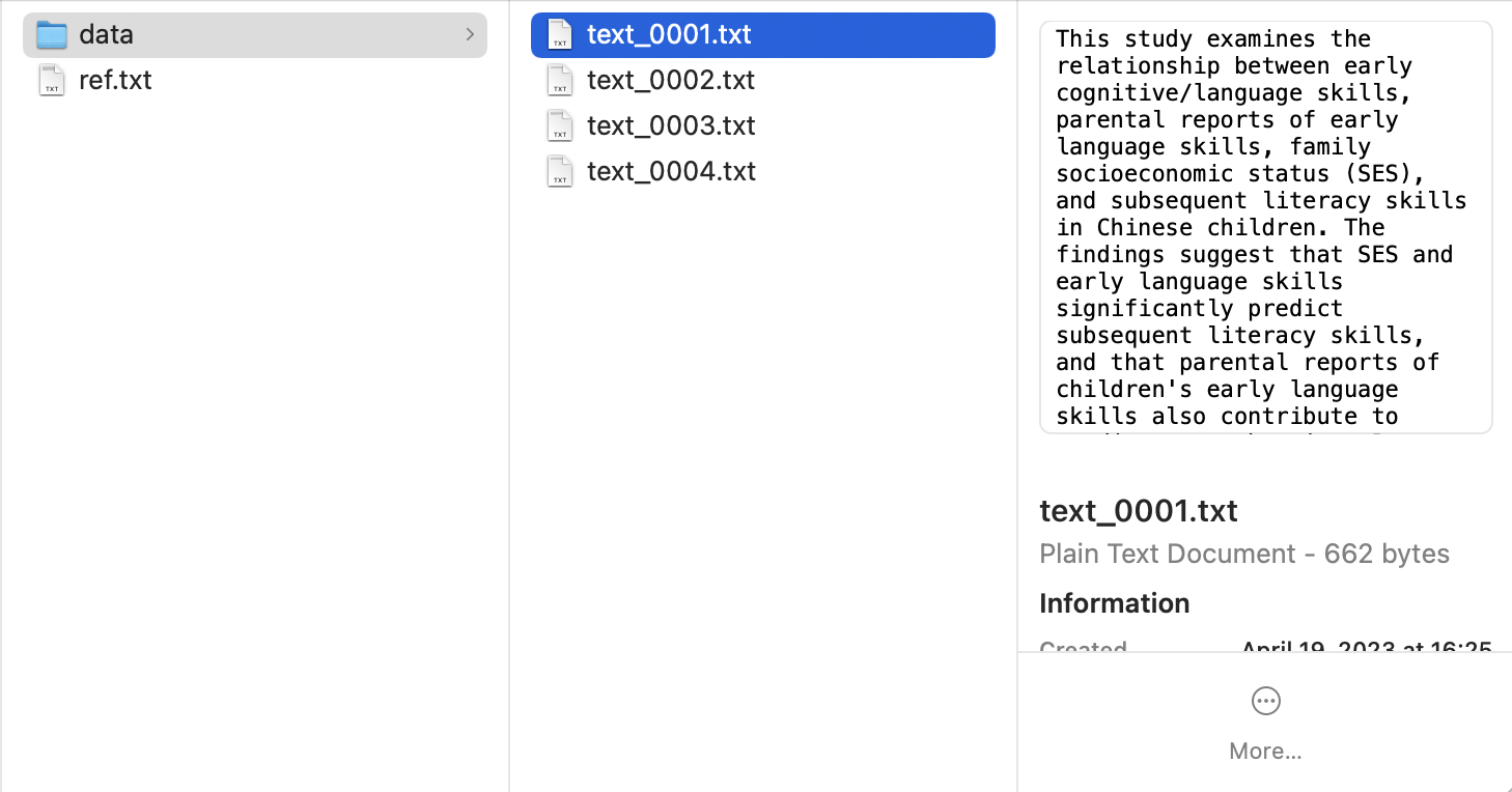
In this example, we have four students’ essays. To use quick_analysis, we need to arrange different students’ essays in separate .txt files and put them in a folder called “data”, while the expert essay (which will be used as the referent network in the calculation) is saved as a file called “ref.txt”. To use quick_analysis, you will need to name the expert data as “ref.txt” exactly. Both the file “ref.txt” and the folder “data” should be included in a parent folder.
Then, you can use the following code for data processing.
import cookiemilk
import numpy as np


# The key-terms. MODIFY IT ACCORDING TO THE KEY-TERMS IN YOUR DATA
key_terms = ['longitudinal prediction',
             'literacy development',
             'cognitive skills',
             'language skills',
             'parental reports',
             'reading achievement']

# The parameters
my_data = cookiemilk.quick_analysis(
    # the file path of the data
    folder='/Users/weiziqian/Desktop/test/text',  # the folder containing ref.txt and students' data. MODIFY IT ACCORDING TO THE FILE PATH OF YOUR DATA

    # about students' data
    data_type='text',  # data type, can be "proposition", "array" or "text". MODIFY IT ACCORDING TO THE CHARACTERISTICS OF YOUR DATA
    key_terms=key_terms,  # key-terms
    synonym=None,  # you can define synonyms here
    as_lower=True,  # whether convert all the alphabetical strings into lowercase. MODIFY IT ACCORDING TO THE CHARACTERISTICS OF YOUR DATA
    pfnet=True,  # whether converting data into PFNets
    max=1.1,  # a parameter of the pathfinder algorithm. MODIFY IT ACCORDING TO THE CHARACTERISTICS OF YOUR DATA
    min=0.1,  # a parameter of the pathfinder algorithm. MODIFY IT ACCORDING TO THE CHARACTERISTICS OF YOUR DATA
    r=np.inf,  # a parameter of the pathfinder algorithm
    encoding='utf-8',  # the encoding format of data files. MODIFY IT ACCORDING TO THE TYPE OF YOUR .TEX FILES
    read_from=0,  # which line should the content in data files be read from. MODIFY IT ACCORDING to THE CHARACTERISTICS OF YOUR DATA

    # about the expert data, the parameters are as same as the above
    referent_type='text',
    r_key_terms=key_terms,
    r_synonym=None,
    r_as_lower=True,  # MODIFY IT ACCORDING TO THE CHARACTERISTICS OF YOUR DATA
    r_pfnet=True,
    r_max=1.1,  # MODIFY IT ACCORDING TO THE CHARACTERISTICS OF YOUR DATA
    r_min=0.1,  # MODIFY IT ACCORDING TO THE CHARACTERISTICS OF YOUR DATA
    r_r=np.inf,  # MODIFY IT ACCORDING TO THE TYPE OF YOUR .TEX FILES
    r_encoding='utf-8',
    r_read_from=0,  # MODIFY IT ACCORDING to THE CHARACTERISTICS OF YOUR DATA

    # Graph-based features calculation (all available features are listed below)
    calculation=[
        'density',  # graph density
        'GC', # holistic graph centrality
        's_density',  # similarity of graph density between students' KSs and the expert KS
        's_GC',  # similarity of graph centrality between students' KSs and the expert KS
        's_surface',  # similarity of surface similarity between students' KSs and the expert KS
        's_concept',  # similarity of conceptual similarity between students' KSs and the expert KS
        's_link',  # similarity of propositional similarity between students' KSs and the expert KS
        's_graphical',  # similarity of graphical similarity between students' KSs and the expert KS
        's_semantic'  # similarity of balanced semantic similarity between students' KSs and the expert KS
    ],
    alpha=0.5,  # a parameter of Tversky's similarity

    # Visualization
    save_figures=True,  # whether to save the visualized graphs
    canvas_size=(500, 500),  # the canvas size
    node_font='sans-serif',  # the font style for node labels
    node_fontsize=12,  # the font size for node labels
    node_fontcolour='black',  # the font color for node lebels
    node_fillcolour='lightgrey',  # the node color
    node_size=12,  # the node size
    edge_colour='lightgrey',  # the edge color
    edge_size=2,  # the edge size
    edge_distance=100,  # the edge distance
    charge=-300,  # the charge force in d3.js
    window_size=(600, 600),  # the window size in pywebview

    # The average graph
    save_average_figures=True,  # whether to generate the average graph
    n_core=None  # the number of core concepts
)
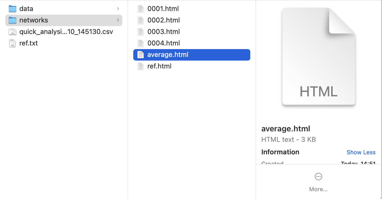
After running the code, we can find a new folder called “networks”, which containing all visualized graphs and the average graph (if you chose to generate it), and a table file called “quick_analysis_20230710_145130.csv” (the numbers indicate the date and time).
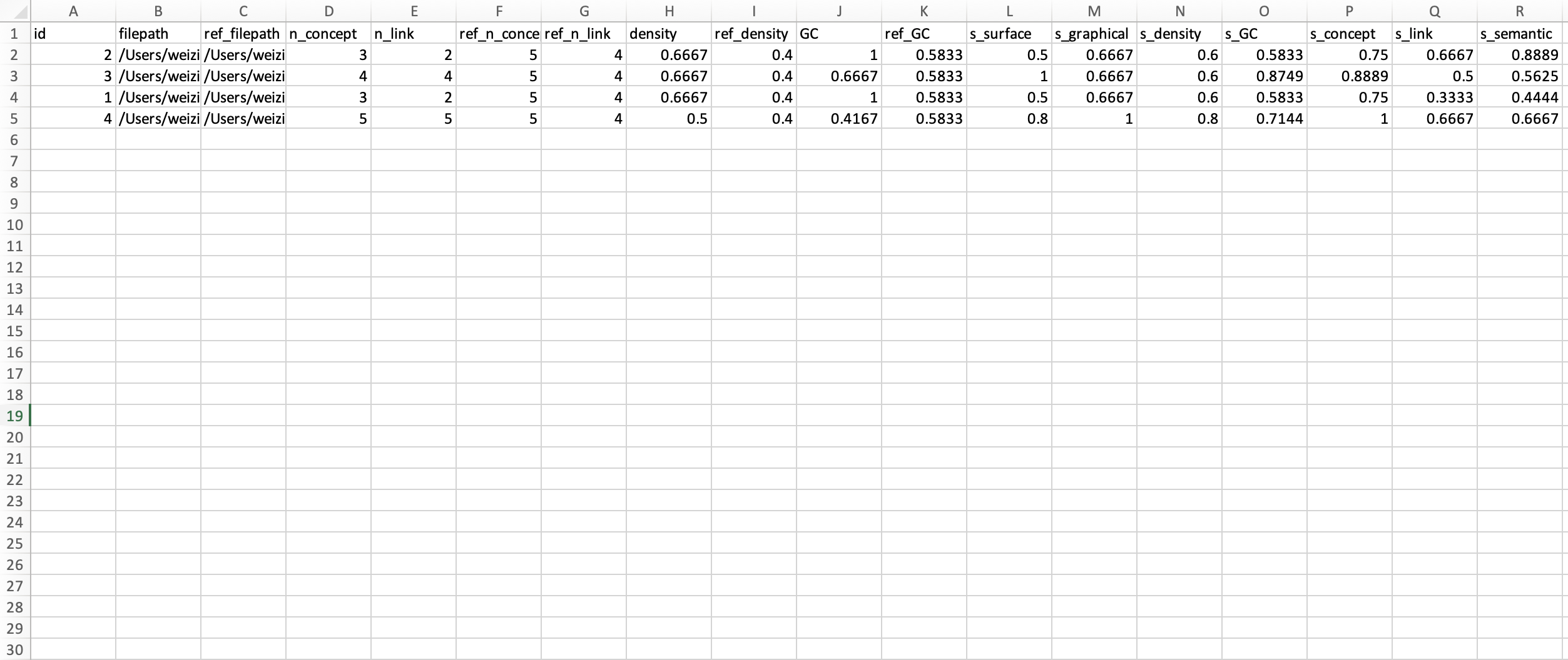
As shown below, the table file contains the basic information (e.g., the number of concepts, the number of links) and results of the features calculation.
3.2 About graph centrality
In this part, I will show you how to calculate graph centrality by hand so that you can understand how the holistic structure of a graph is estimated. And then I will show you how to use the function calc_gcent to calculate graph centrality conveniently.
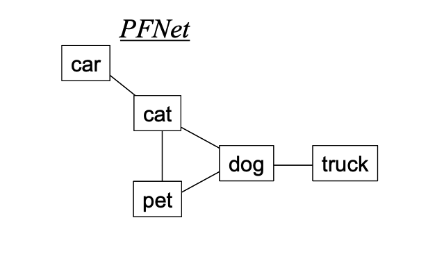
We will use an example network from Clariana and Koul’s research (2004). Please see below. This network includes five nodes and five edges (i.e., links).
Calculate graph centrality manually
The equations of graph centrality are shown below (Clariana, Rysavy, & Taricani, 2015).
Equation 1: CD(v) = deg(v) / (n – 1)
Equation 2: CD(G) = ∑vi=1 [max(CD(vi)) – CD(vi)] / (n – 2)
First, we need to calculate the node degree of each node. In graph theory, the degree of a node is the number of edges (i.e., links) including the node. In this example, the node “dog” connects to three other nodes. Considering “dog” has three links (i.e., “dog-cat”, “dog-pet”, “dog-truck”), we can say deg(“dog”) = 3. Similar to this, other nodes’ degrees can be calculated as follows.
deg(“cat”) = 3
deg(“dog”) = 3
deg(“pet”) = 2
deg(“car”) = 1
deg(“truck”) = 1
Second, we need to calculate node centrality for each node. Based on Equation 1, each node’s centrality can be calculated as follows.
CD(“cat”) = deg(“cat”)/(n - 1) = 3/(5 - 1) = 0.75
CD(“dog”) = deg(“dog”)/(n - 1) = 3/(5 - 1) = 0.75
CD(“pet”) = deg(“pet”)/(n - 1) = 2/(5 - 1) = 0.50
CD(“car”) = deg(“car”)/(n - 1) = 1/(5 - 1) = 0.25
CD(“truck”) = deg(“truck”)/(n - 1) = 1/(5 - 1) = 0.25
Third, we then use Equation 2 to calculate the holistic centrality of the network (i.e., graph centrality) as follows. Note that the highest node centrality in this network is 0.75, so max(C~D~(v~i~)) = 0.75.
CD(G) = [(0.75 - 0.75) + (0.75 - 0.75) + (0.75 - 0.50) + (0.75 - 0.25) + (0.75 - 0.25)] / (5 - 2) = 0.4267
As result, C~D~(G) of this PFNet is 0.4267. I hope this example is useful for you to understand the calculation of graph centrality.
Use calc_gcent to calculate graph centrality
Finally, let’s try to use calc_gcent to calculate the graph centrality of this PFNet automatically.
import cookiemilk

# import the example PFNet
my_cmap1 = [['car', 'cat'], ['cat', 'pet'], ['cat', 'dog'], ['pet', 'dog'], ['dog', 'truck']]
my_data1 = cookiemilk.cmap2graph(file=my_cmap1, data_type='pair', read_from_file=False)

# calculation
my_results = cookiemilk.calc_gcent(my_data1, detailed=True)
And here are the results. We have set the argument detailed=True, which will enable us to check each step of the calculation. When analyzing data, you can set the argument detailed=False to avoid redundant outputs.
adjacency matrix:
 [[0. 1. 0. 0. 0.]
 [1. 0. 1. 1. 0.]
 [0. 1. 0. 1. 0.]
 [0. 1. 1. 0. 1.]
 [0. 0. 0. 1. 0.]]
n: 5
node_degree: [1. 3. 2. 3. 1.]
ncent: [0.25 0.75 0.5  0.75 0.25]
gcent: 0.41666666666666663
As the results are stored in the variable my_results, we can also print it to see the value of graph centrality.
print(my_results)
And the output is shown below.
0.41666666666666663
References
Clariana, R. B., & Koul, R. (2004). A computer-based approach for translating text into concept map-like representations. In A. J. Canas, J. D. Novak, and F. M. Gonzales, Eds., Concept maps: theory, methodology, technology, vol. 2, in the Proceedings of the First International Conference on Concept Mapping, Pamplona, Spain, Sep 14-17, pp.131-134.
Clariana, R. B., Rysavy, M. D., & Taricani, E. (2015). Text signals influence team artifacts. Educational Technology Research and Development, 63(1), 35-52.
3.3 Generate expert models via word embedding methods
Here I will show you some examples of construting KSs with specific key-terms using word embedding methods.
First, open the website http://wordvec.colorado.edu. You can also find basic information and the literature about Latent Semantic Analysis (LSA), word2vec and BERT from the website. These are the three approaches used in the following examples.
we can click “Matrix Comparison” and then select arguments, input key-terms (I used the example key-terms in “Part 2 A quick start”) and submit. The similarity matrix will be presented.
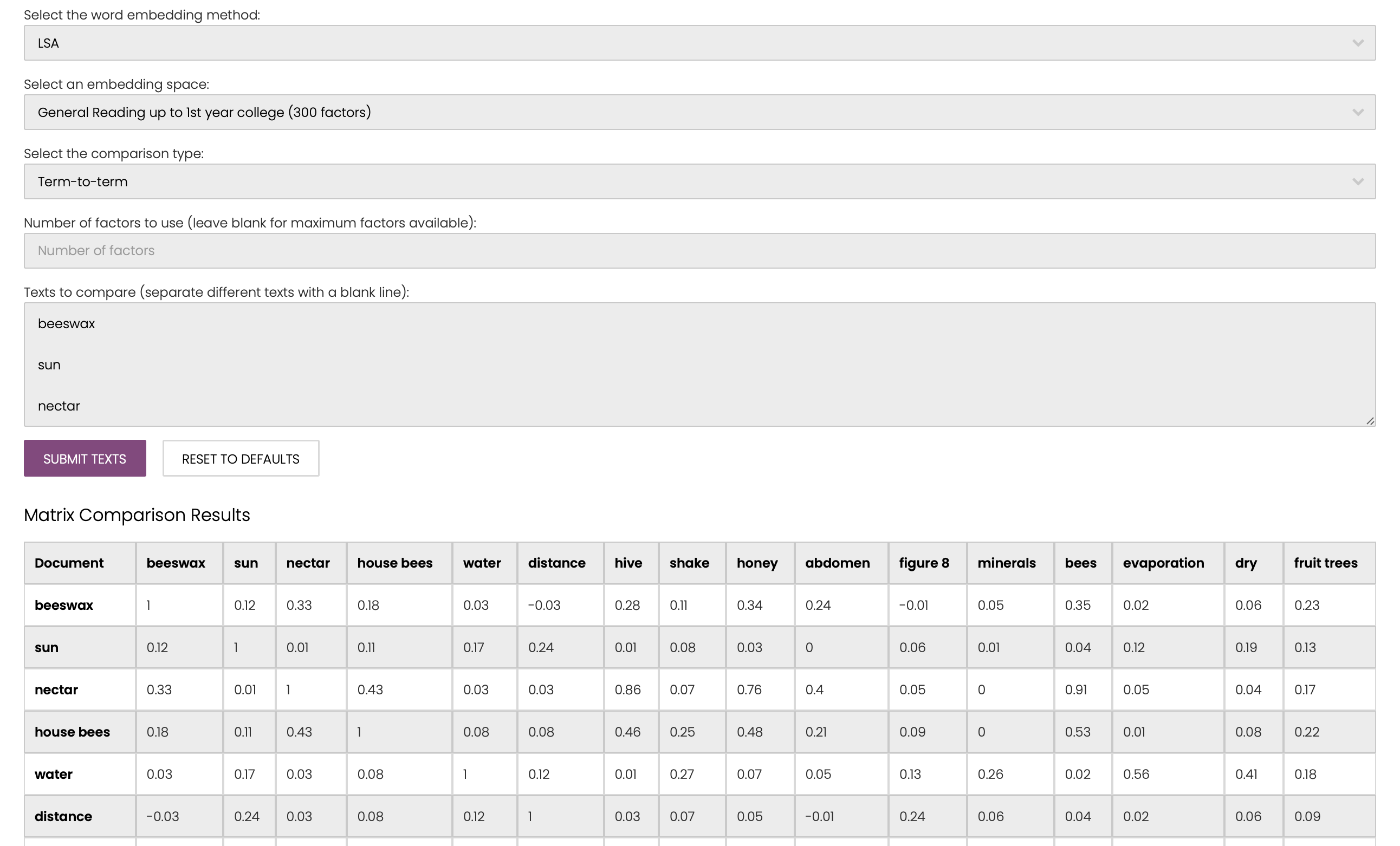
We can then save each matrix in seperate .prx file and use the following code to convert them into PFNets.
import cookiemilk
# the document model
text = 'Bees make honey to survive. It is their only essential food. If there are 60,000 bees in a hive about one ' \
'third of them will be involved in gathering nectar which is then made into honey by the house bees. A small ' \
'number of bees work as foragers or searchers. They find a source of nectar, then return to the hive to tell ' \
'the other bees where it is. Foragers let the other bees know where the source of the nectar is by performing ' \
'a dance which gives information about the direction and the distance the bees will need to fly. During this ' \
'dance the bee shakes her abdomen from side to side while running in circles in the shape of a figure 8. The ' \
'dance follows the pattern shown on the following diagram. The diagram shows a bee dancing inside the hive on ' \
'the vertical face of the honeycomb. If the middle part of the figure 8 points straight up it means that bees ' \
'can find the food if they fly straight towards the sun. If the middle part of the figure 8 points to the ' \
'right, the food is to the right of the sun. The distance of the food from the hive is indicated by the length ' \
'of time that the bee shakes her abdomen. If the food is quite near the bee shakes her abdomen for a short ' \
'time. If it is a long way away she shakes her abdomen for a long time. When the bees arrive at the hive ' \
'carrying nectar they give this to the house bees. The house bees move the nectar around with their mandibles, ' \
'exposing it to the warm dry air of the hive. When it is first gathered the nectar contains sugar and minerals ' \
'mixed with about 80% water. After ten to twenty minutes, when much of the excess water has evaporated, ' \
'the house bees put the nectar in a cell in the honeycomb where evaporation continues. After three days, ' \
'the honey in the cells contains about 20% water. At this stage, the bees cover the cells with lids which they ' \
'make out of beeswax. At any one time the bees in a hive usually gather nectar from the same type of blossom ' \
'and from the same area. Some of the main sources of nectar are fruit trees, clover and flowering trees. '
key_terms = ['beeswax', 'sun', 'nectar', 'house bees', 'water', 'distance',
'hive', 'shake', 'honey', 'abdomen', 'figure 8', 'minerals',
'bees', 'evaporation', 'dry', 'fruit trees']
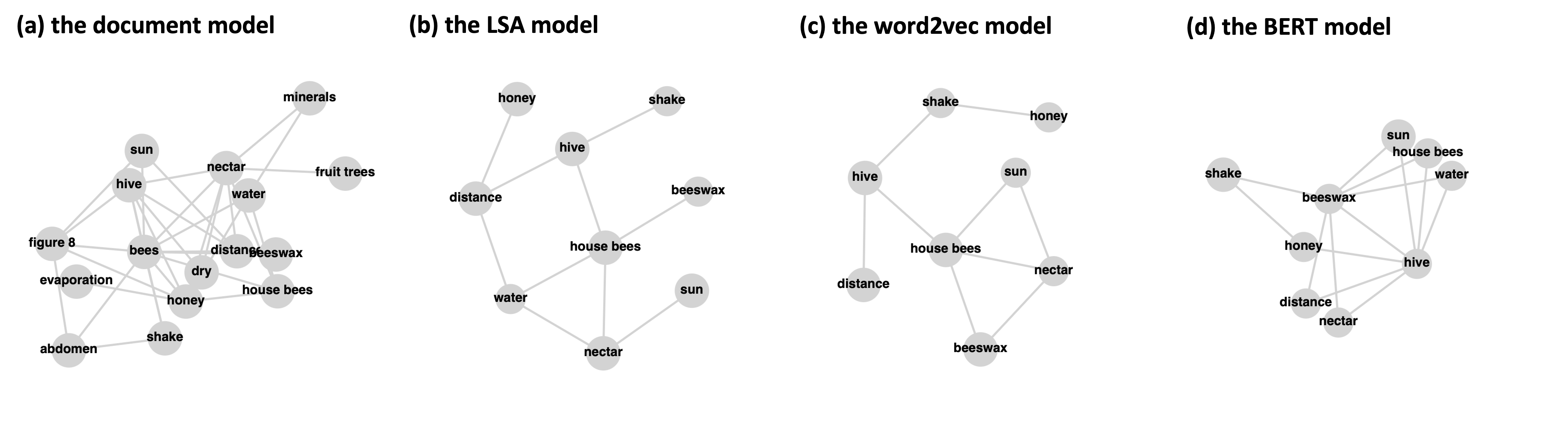
bees_text = cookiemilk.text2graph(data=text, key_terms=key_terms, as_lower=True, read_from_file=False)
# the LSA model
bees_lsa = cookiemilk.cmap2graph(data='/Users/weiziqian/Desktop/test/word_embedding/data/lsa.prx',
data_type='array', key_terms=key_terms, read_from_file=True, read_from=0,
pfnet=True, max=1.1, min=0.1)
bees_w2v = cookiemilk.cmap2graph(data='/Users/weiziqian/Desktop/test/word_embedding/data/w2v.prx',
data_type='array', key_terms=key_terms, read_from_file=True, read_from=0,
pfnet=True, max=1.1, min=0.1)
bees_bert = cookiemilk.cmap2graph(data='/Users/weiziqian/Desktop/test/word_embedding/data/bert.prx',
data_type='array', key_terms=key_terms, read_from_file=True, read_from=0,
pfnet=True, max=1.1, min=0.1)
# save visualized graphs
cookiemilk.draw(graph=bees_text, show=False, save=True, filename="fig_text")
cookiemilk.draw(graph=bees_lsa, show=False, save=True, filename="fig_lsa")
cookiemilk.draw(graph=bees_w2v, show=False, save=True, filename="fig_w2v")
cookiemilk.draw(graph=bees_bert, show=False, save=True, filename="fig_bert")
And here are the visualized models. You may notice that some key-terms disappear in the latter three models. This is because there are no related edges after performing the pathfinder algorithm, and thus these nodes are ignored. Because we used different corpora in different approaches, these models cannot be compared directly. However, the examples show that word-embedding models are more concise and possibly can be used as automatically generated expert references.